Top Data Science Interview Questions and Answers (2026 Guide)

Below is a list of the most common questions asked in data science interviews, covering topics in statistics, machine learning (ML) coding, and SQL.

The list was compiled with real questions from data science candidates and input from senior data scientists and machine learning engineers at Amazon, Google, Tinder, BCG, and Instacart.

👋

Want to become a data scientist? This guide contains excerpts from Exponent's complete data science and machine learning interview prep courses.

Sneak peek:
- Watch a Tinder DS answer: Determine the sample size for an experiment.
- Watch a senior DS answer: What is a P-value?
- Practice yourself: Predict results from a fair coin flip.

Haziqa Sajid, an advocate for ML and data science developers, wrote this post. Raj Singh, a senior machine learning engineer at Amazon and interview coach, reviewed it.

Statistics and Experimentation

Statistical experimentation is a key component of data science.

This interview section assesses your understanding of statistical concepts and ability to analyze data using statistical methods.

What to expect

The statistics portion of the interview typically includes three types of questions:

Numerical: Solve a mathematical problem.
Conceptual: Demonstrate your understanding of core statistics and experimentation principles.
Applied: Choose the best statistical approach to solve a given real-world problem.

Here are some examples of common interview questions:

1. What are the measures of central tendency? Explain the significance of each.

Measures of central tendency describe the center of a data distribution.

These descriptive statistics summarize data based on its numerical values. The three most common measures are:

Mean: The average of all values in a dataset. It reflects the central value by considering the magnitude of each data point. The mean is useful when you need a single number to describe a series, like the average height in a study. However, it is sensitive to outliers, which can skew the result.
Median: The middle value in a sorted dataset. Unlike the mean, outliers do not affect the median, making it a good alternative when the data contains extreme values.
Mode: The most frequently occurring value in a dataset. It helps identify the most common data point and works for numerical and categorical data.

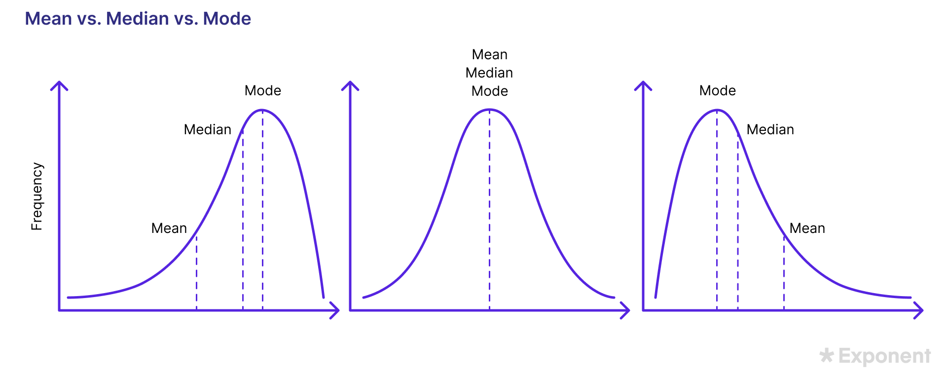
2. In a positively skewed distribution, which measure of central tendency would likely be larger: the mean or the median? Why?

A positively skewed distribution has a larger tail towards the right.

The longer tail means the distribution contains extreme values (outliers) that stretch it to the right. In such a case, the median of a series is unaffected; however, the mean is sensitive to outliers.

Hence, it is more likely to be large in positively skewed data.

3. Explain the concept of correlation between two variables. How would you interpret a correlation value of +0.8?

Correlation describes a linear relationship between two variables, X and Y.

It is a standardized value that provides the direction and magnitude of the relationship. The correlation value is bound between -1 and +1, where -1 means the variables are perfectly opposite.

When one increases in value, the other decreases by the same amount, and vice versa for +1.

A correlation of 0 means the two variables are entirely independent.

A correlation of +0.8 means that the two variables have an almost perfectly positive correlation. 0.8 indicates that when X increases by a particular value, Y will gain 80% of the increase of X.

4. How would you detect outliers in your data?

Outliers are extreme values that deviate from the overall pattern in the data. In data science, they are often flagged as anomalies and removed before further analysis.

A common method of detecting outliers is the 1.5 interquartile range (IQR) rule. This involves calculating the data's 1st quartile (25th percentile) and 3rd quartile (75th percentile).

Outliers are defined as any values that fall below 1.5 times the IQR below the 1st quartile or above 1.5 times the IQR above the 3rd quartile.

ℹ️

This question was asked at FanDuel. “How would you design an ML monitoring system for a fantasy sports app. Take into account outliers, data quality, and drift.”

5. Design a hypothesis test.

A hypothesis test follows a standard 7-step process.

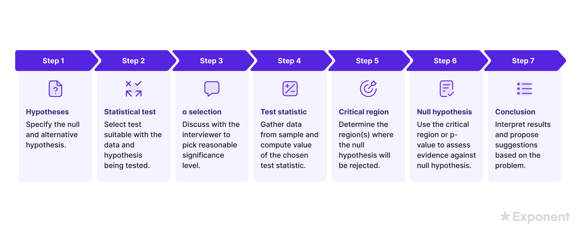
Learn how to answer hypothesis testing questions.

Formulate hypotheses: Define the null and alternative hypotheses.
Select the test: Choose the most appropriate statistical test for the data and hypothesis.
Set a significance level: A 0.05 significance level (alpha) is typically used.
Calculate the test statistic: Collect sample data and compute the test statistic.
Determine the critical region: Identify the conditions under which the null hypothesis will be rejected.
Evaluate the null hypothesis: Assess evidence using the critical region or p-value.
Interpret results: Explain the implications and provide recommendations based on the findings.

6. Can you explain a p-value?

A p-value represents the probability of obtaining a test statistic at least as extreme as the observed one, assuming the null hypothesis is true.

A p-value less than 0.05 suggests the result is unlikely due to chance, leading to rejection of the null hypothesis. A higher p-value indicates that the observed data is consistent with the null hypothesis.

Learn more about core probability concepts.

7. What's the difference between a Type I and a Type II error?

Type I and Type II errors occur in hypothesis testing:

Type I error (false positive): Rejecting the null hypothesis when it is actually true. The probability of this error is denoted by alpha (α).
Type II error (false negative): Failing to reject the null hypothesis when it is actually false. The probability of this error is denoted by beta (β).

Reducing one error increases the likelihood of the other, requiring a balance between the two.

8. What's the central limit theorem, and how does it relate to hypothesis testing?

The central limit theorem (CLT) states that as the sample size increases, the distribution of the sample means approaches the population mean, forming a normal distribution.

This is crucial in hypothesis testing because it allows data scientists to confidently generalize results from a sample to the entire population, assuming a normal distribution for many statistical tests.

9. What does the confidence level mean when building a confidence interval?

A confidence interval defines the range within which we expect a population parameter to fall when repeating an experiment using random samples.

The confidence level represents the probability that the true value falls within the interval. For example, a 95% confidence level means that if the experiment is repeated 100 times, the true value will fall within the confidence interval 95 times.

There is a trade-off between the confidence interval and confidence level: Narrowing the interval increases precision but lowers the confidence level, reducing it from 95% to 90%.

Data Communication and Case Studies

During your interview, expect questions about your past projects and situational scenarios.

These questions are designed to evaluate your problem-solving approach, assess your experience, and gauge your communication and presentation skills. Common questions include:

10. Walk us through one of your most exciting data science projects.

This question assesses your experience based on your chosen project and how effectively you explain it.

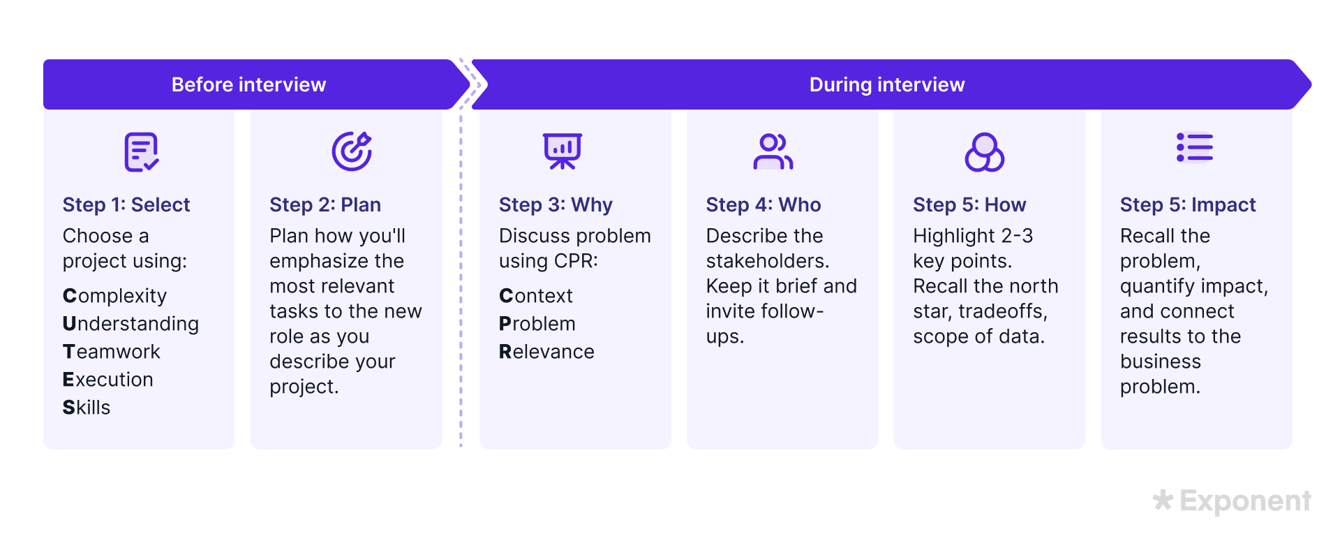
Interviewers will focus on:

Complexity: The difficulty of the project.
Understanding: Your grasp of the data science principles at play.
Teamwork: How well you collaborate with others cross-functionally.
Execution: Your decision-making process.
Skills: The relevant skills you demonstrated and how they align with the job.

Choose a project that aligns with the role you're applying for, highlighting the skills that will benefit the potential employer.

Show how your experience is a good fit for their ongoing projects.

11. How would you investigate a sudden viewer drop at Meta?

This situational question tests your ability to break down a problem and solve it step by step.

ℹ️

Watch a mock interview with a Tinder data scientist: "Investigate a sudden viewer drop at Meta."

Here’s an approach:

Clarify assumptions and scope: Clarify what “Viewer Drop” means. Is it specific to certain pages or the entire app? Does it affect all users or just a specific region?
Analyze the trend: Determine if the drop is sudden or gradual. A sudden drop may indicate an unusual event, while a gradual decline could point to a pattern that needs further investigation. Also, check for seasonal patterns.
Compare metrics: Investigate if other metrics, like likes or comments, have declined.
Identify the root cause: Consider whether external factors (e.g., a new competitor) or internal issues (e.g., product changes) might drive the drop.

Following this framework will help you diagnose and address the issue.

12. How would you use data to help Snap Engineering measure, evaluate, and improve phone camera speed?

This scenario challenges you to identify how data can improve a widely used application.

ℹ️

Watch a mock interview with a Snap data scientist: "Use data to improve Snap's camera."

Here’s a suggested approach:

Measure camera speed: Begin by identifying factors influencing camera speed, such as the device type and internet quality. Analyze these factors by looking at percentiles, e.g., how fast the app loads for 50% of users.
Ensure data quality: Make sure the data collected from different devices is clean and reliable. Any anomalies should be processed or removed.
Leverage A/B testing: Use A/B testing to collect user feedback and evaluate new features. A feedback loop based on user input can help refine features and monitor long-term performance.

This approach emphasizes the use of data-driven insights to improve user experience.

Python

Python is a core programming language for data scientists and is featured in nearly every data science interview.

Python-based coding questions assess your ability to manipulate data and familiarity with popular frameworks like Pandas.

Some common questions include:

13. Given the DataFrame below, write a solution to fetch the three lowest-earning employees, including their IDs, names, and salaries.

This entry-level question tests your ability to work with DataFrames in Python.

id	first_name	last_name	salary	department_id
int	varchar	varchar	int	int

Here’s a pseudo-code solution using Pandas:

Python

import pandas as pd

def lowest_earning_employees(employees: pd.DataFrame) -&gt; pd.DataFrame:
    # Select relevant columns
    selected_columns = employees[['id', 'first_name', 'last_name', 'salary']]

    # Sort by salary in ascending order
    sorted_employees = selected_columns.sort_values(by='salary', ascending=True)

    # Limit to the first 3 entries (the lowest 3 salaries)
    lowest_earning_employees = sorted_employees.head(3)

    return lowest_earning_employees

This medium-level question assesses your ability to manage data across multiple DataFrames.

The task requires joining the correct tables and extracting the desired result.

users

id	first_name	last_name	user_city	email
int	varchar	varchar	int	int

transactions

id	customer_id	product_id	amount	currency_code	date
int	int	int	int	varchar	date

products

id	name	product_line_id	stock
int	varchar	int	int

product_lines

id	name
int	varchar

exchange_rate

id	source_currency_code	target_currency_code	rate
int	varchar	varchar	numeric

Here’s a pseudo-code solution using Pandas:

Python

import pandas as pd

def find_revenue_by_city(transactions: pd.DataFrame,
                         users: pd.DataFrame,
                         exchange_rate: pd.DataFrame) -&gt; pd.DataFrame:
    # Merge Transactions with Users
    transactions_with_users = pd.merge(transactions, users, left_on='customer_id', right_on='id')

    # Merge non-USD transactions with exchange rates
    transactions_with_exchange = pd.merge(
        transactions_with_users,
        exchange_rate[exchange_rate['target_currency_code'] == 'USD'],
        how='left',
        left_on='currency_code',
        right_on='source_currency_code'
    )

    # Assign an exchange rate of 1.0 for USD transactions
    transactions_with_exchange['rate'] = transactions_with_exchange['rate'].fillna(1.0)

    # Calculate the amount in USD
    transactions_with_exchange['amount_usd'] = transactions_with_exchange['amount'] * transactions_with_exchange['rate']

    # Aggregate revenue by city
    revenue_by_city = transactions_with_exchange.groupby('user_city')['amount_usd'].sum().reset_index()

    # Sort by revenue
    revenue_by_city = revenue_by_city.sort_values(by='amount_usd', ascending=False).reset_index(drop=True)

    # Rename columns for clarity
    revenue_by_city.columns = ['user_city', 'total_revenue']

    return revenue_by_city

15. You are given a table with varying distances between different pairs of cities recorded by GPS systems. The table includes columns: origin, destination, and distance. Write a function to calculate the average distance between each pair of cities and return a new table with the columns `city_pair` and `average_distance`. The `city_pair` column should list the cities in alphabetical order (e.g., “CityA-CityB”), and the `average_distance` should be rounded to two decimal places. Sort the results by `average_distance` in ascending order.

This medium-difficulty question tests your ability to aggregate and manipulate data.

Here’s a pseudo-code solution using Pandas:

Python

import pandas as pd

def find_average_distance(gps_data: pd.DataFrame) -&gt; pd.DataFrame:
    # Create a new column with city pairs in alphabetical order
    gps_data['city_pair'] = gps_data.apply(
        lambda row: '-'.join(sorted([row['origin', 'destination']])), axis=1
    )

    # Group by the city pair and calculate the average distance
    result = gps_data.groupby('city_pair')['distance'].mean().reset_index()

    # Round the average distances to two decimal places
    result['distance'] = result['distance'].round(2)

    # Rename columns
    result.columns = ['city_pair', 'average_distance']

    # Sort by average_distance in ascending order
    result = result.sort_values(by='average_distance').reset_index(drop=True)

    return result

16. Given the DataFrame format below, write a function to identify the user who liked a post the quickest after logging in.

This difficult question assesses your advanced data manipulation skills, requiring you to work with timestamps and pivot tables.

user_id	event	timestamp
1	login	2024-07-25 10:00:00
1	like	2024-07-25 10:01:10

Here’s a pseudo-code solution using Pandas:

Python

import pandas as pd

def find_fastest_like(log: pd.DataFrame) -&gt; pd.DataFrame:
    # Create pivot table to get the earliest login and like timestamps for each user_id
    pivot_df = pd.pivot_table(
        data=log,
        index='user_id',
        columns='event',
        values='timestamp',
        aggfunc='min'
    ).reset_index()

    # Drop unnecessary columns
    pivot_df.columns.name = None
    pivot_df = pivot_df[['user_id', 'login', 'like']]

    # Calculate the time difference in minutes
    pivot_df['time_between'] = ((pivot_df['like'] - pivot_df['login']).dt.total_seconds() / 60).round().astype(int)

    # Sort by time_between
    pivot_df = pivot_df.sort_values(by=['time_between'])

    # Return the user with the shortest time_between
    result = pivot_df.head(1)

    return result

17. You have a user behavior log, but some records are duplicated, and some timestamps are missing. Since the logs are recorded chronologically, remove duplicates and fill in missing timestamps by interpolating the data.

This medium-level question tests your ability to clean and preprocess data.

Here’s a pseudo-code solution using Pandas:

Python

import pandas as pd

def interpolate_data(log: pd.DataFrame) -&gt; pd.DataFrame:
    # Remove duplicate rows
    log = log.drop_duplicates()

    # Interpolate missing timestamps
    log = log.interpolate(method='linear', limit_direction='forward')

    return log

SQL

Data scientists frequently use SQL to interact with relational databases (RDBMS), and a basic understanding of core SQL functionalities is essential.

SQL interview questions typically focus on functions like JOIN, GROUP BY, and aggregations.

Common questions include:

18. How do you use a GROUP BY clause in SQL? What are some common aggregate functions used with GROUP BY?

The GROUP BY clause groups rows that have the same values in specified columns. It is commonly used with aggregate functions to summarize data. Typical aggregate functions used with GROUP BY include:

SUM
AVG
COUNT
MIN
MAX

Example Syntax:

SQL

SELECT column1, SUM(column2)
FROM table_name
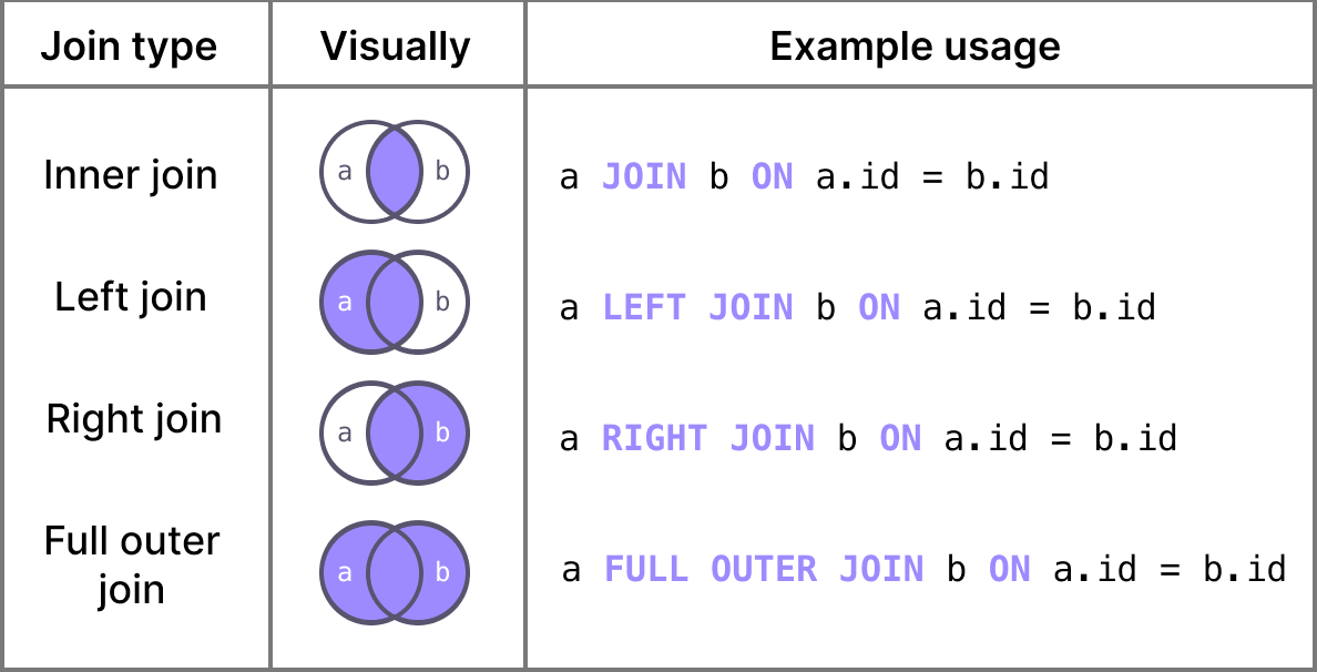
GROUP BY column1;

19. What is a JOIN statement in SQL? Explain the different types of JOINS.

A JOIN clause combines rows from two or more tables based on a related column (key).

The syntax for a JOIN is:

SQL

SELECT *
FROM table1 t1
JOIN table2 t2
ON t1.column = t2.column;

Types of JOIN:

LEFT JOIN: Returns all rows from the left table and matched rows from the right table. Unmatched rows from the right table will have NULL values.
RIGHT JOIN: Returns all rows from the right table and matched rows from the left table. Unmatched rows from the left table will have NULL values.
INNER JOIN: Returns rows where there is a match in both tables.
OUTER JOIN: Returns all rows from both tables. NULL values are returned where there is no match.

20. Write SQL code to show the total number of successful posts per user type in the current month (assumed to be November 2023).

The post and post_user tables have the following schemas. The output should include:

user_type
post_success (number of successful posts)
post_attempt (total number of posts)
post_success_rate (success rate, ranging from 0.00 to 1.00)

Order the results by descending success rate.

This is a medium-level SQL question that tests your ability to use aggregation, GROUP BY, JOIN, and sorting functions. Here’s a pseudo-code solution:

SQL

SELECT
    pu.user_type,
    SUM(p.is_successful_post) AS post_success,
    COUNT(p.is_successful_post) AS post_attempt,
    ROUND(SUM(p.is_successful_post) * 1.0 / COUNT(p.is_successful_post), 2) AS post_success_rate
FROM post AS p
JOIN post_user AS pu ON p.user_id = pu.user_id
WHERE p.post_date BETWEEN '2023-11-01' AND '2023-11-30'
GROUP BY pu.user_type
ORDER BY post_success_rate DESC;

21. An organization has conducted SQL tests for its backend developers. A developer may attempt a test multiple times. The organization wants to calculate each developer's total score by summing the maximum scores from all tests. Only the maximum score is considered if a developer has attempted the same test multiple times. If multiple developers have the same total score, sort the results by employee ID in ascending order.

This medium-difficulty question requires knowledge of basic SQL concepts, including joins and aggregations.

Here's a pseudo-code solution using SQL:

SQL

SELECT
    e.id AS employee_id,
    e.name AS employee_name,
    SUM(max_score) AS total_score
FROM employees e
INNER JOIN (
    SELECT employee_id, MAX(score) AS max_score
    FROM test_results
    GROUP BY employee_id, test_id
) r
ON r.employee_id = e.id
GROUP BY e.id, e.name
ORDER BY total_score DESC, e.id ASC;

22. What are window functions in SQL? Explain their syntax and usage.

Window functions are advanced SQL tools that perform calculations across a set of rows related to the current row.

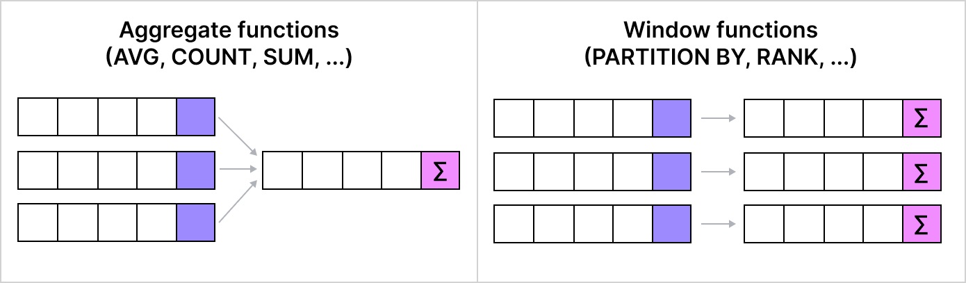
Learn more about window functions and adjusting window size.

They allow operations over partitions of data without collapsing rows into groups.

Common window functions include:

RANK
DENSE RANK
ROW NUMBER

Basic syntax:

SQL

SELECT column1, column2,
    RANK() OVER (PARTITION BY column1 ORDER BY column2 DESC) AS window_column
FROM table_name;

In this example, the RANK() function assigns a rank to each row within the partitions defined by column1. The rank resets for each new partition.

23. Order departments by revenue over the last 12 months, showing `department_name` and `total_revenue`.

This medium-difficulty question tests your ability to join tables and aggregate revenue. The solution uses a join to connect customer orders with departments and aggregates the order amounts.

SQL

SELECT
    d.department_name,
    SUM(o.order_amount) AS total_revenue
FROM departments d
JOIN orders o ON d.department_id = o.department_id
WHERE o.order_date &gt;= date('now', '-12 months')
GROUP BY d.department_name
ORDER BY total_revenue DESC;

24. Write an SQL query to calculate the total transaction value in USD for the product line "Telephones" and return it as `total_amount_in_dollars`. You will need to convert non-USD amounts using the exchange rate and ensure proper scaling of the values.

This is a difficult question that involves complex joins and calculations. Here's a pseudo-code solution:

SQL

WITH base AS (
    SELECT
        t.product_id,
        CASE
            WHEN t.currency_code = 'USD' THEN t.amount / 100.0
            ELSE t.amount / 100.0 * er.rate
        END AS amount_in_usd
    FROM transactions t
    LEFT JOIN exchange_rate er
        ON t.currency_code = er.source_currency_code AND er.target_currency_code = 'USD'
    INNER JOIN products p
        ON t.product_id = p.id
    INNER JOIN product_lines pl
        ON p.product_line_id = pl.id AND pl.name = 'Telephones'
)
SELECT
    ROUND(SUM(amount_in_usd), 2) AS total_amount_in_dollars
FROM base;

25. Given the `orders` table, write an SQL query that returns the `order_id`, `status`, `start_date`, and `end_date` for each status period of an order. If a status is the first for that order, `end_date` should be `NULL`.

This hard-difficulty question requires date-wise calculations. A common table expression (CTE) helps calculate the relevant fields. Here's a pseudo-code solution:

SQL

WITH StatusChanges AS (
    SELECT
        order_id,
        order_date,
        status,
        LEAD(order_date) OVER(PARTITION BY order_id ORDER BY order_date) AS next_date,
        LAG(status) OVER(PARTITION BY order_id ORDER BY order_date) AS prev_status
    FROM orders
)
SELECT
    order_id,
    status,
    order_date AS start_date,
    next_date AS end_date
FROM StatusChanges
WHERE status != prev_status OR prev_status IS NULL;

ML Coding

The machine learning coding interview will judge your theoretical concepts and how well you can demonstrate them via a practical application.

You can expect questions that will:

Test your knowledge of the core concepts of machine learning.
Test your familiarity with popular frameworks like Sk-Learn and Keras.
Judge your understanding and implementation of popular machine learning algorithms.

Some common questions to expect are:

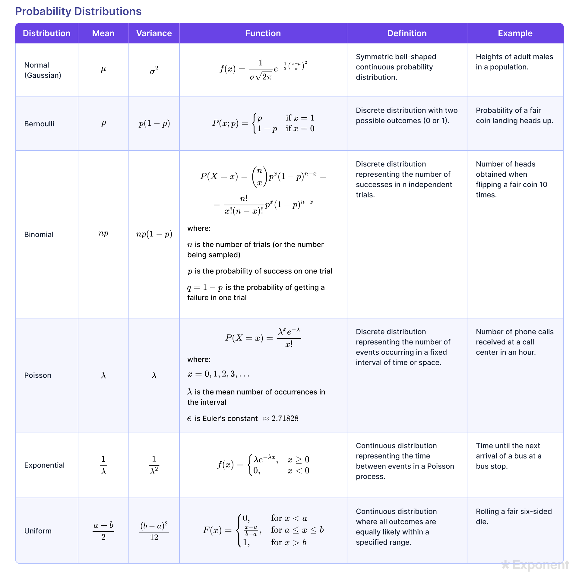
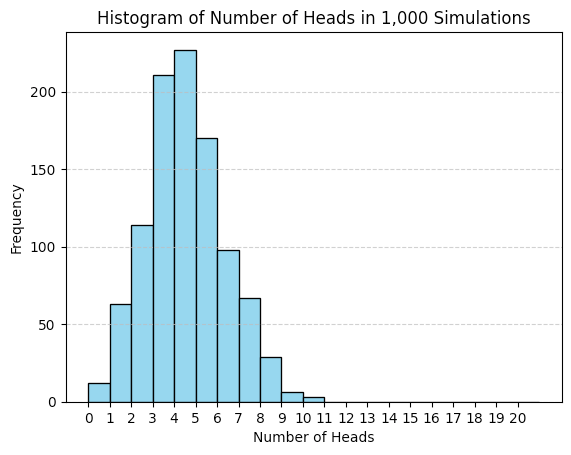
26. Write a function to simulate flipping a biased coin 20 times in each of 1,000 simulations, where each flip has a 20% chance of landing heads. Then, create a histogram showing the distribution of the number of heads observed in these 1,000 simulations.

A coin flip can be simulated in many ways in Python.

However, the most straightforward approach would be to use a binomial distribution.

A binomial distribution models the likelihood of achieving a particular outcome in an experiment, such as getting heads when flipping a coin.

Next, we need to plot the results as a histogram. Python libraries like Matplotlib or Plotly can be used to visualize this.

This is a pseudo-code solution using Python.

Python

import numpy as np
import matplotlib.pyplot as plt

def simulate_coin_flips(n_simulations, n_flips, p_head):
    """Simulate flipping a coin n_flips times in each of n_simulations simulations."""
    results = np.random.binomial(n_flips, p_head, n_simulations)
    return results

sim_results = simulate_coin_flips(1000, 20, 0.2)

# Create histogram
plt.hist(sim_results, bins=range(20 + 2), edgecolor='black', color='skyblue')
plt.title('Histogram of Number of Heads in 1,000 Simulations')
plt.xlabel('Number of Heads')
plt.ylabel('Frequency')
plt.xticks(range(20 + 1))
plt.grid(axis='y', linestyle='--', alpha=0.7)
plt.show()

27. Implement the KMeans clustering algorithm from scratch in Python.

K-means is a popular clustering algorithm that uses an iterative approach to identify n centroids in the data.

The centroids are the central points of each of the n clusters.

In k-means, the centroids represent the average value of the entire cluster and are used to classify a new data point into one of the clusters.

This is a pseudo-code solution using Python:

Python

import numpy as np

class Centroid:
  def __init__(self, location, vectors):
      self.location = location  # (D,)
      self.vectors = vectors    # (N_i, D)

class KMeans:
  def __init__(self, n_features, k):
      self.n_features = n_features
      self.centroids = [
          Centroid(
              location=np.random.randn(n_features),
              vectors=np.empty((0, n_features))
          )
          for _ in range(k)
      ]

  def distance(self, x, y):
      return np.sqrt(np.dot(x - y, x - y))

  def fit(self, X, n_iterations):
      for _ in range(n_iterations):
          # start initialization over again
          for centroid in self.centroids:
              centroid.vectors = np.empty((0, self.n_features))

          for x_i in X:
              distances = [
                  self.distance(x_i, centroid.location) for centroid in self.centroids
              ]

              min_idx = distances.index(min(distances))
              cur_vectors = self.centroids[min_idx].vectors

              self.centroids[min_idx].vectors = np.vstack((cur_vectors, x_i))

          for centroid in self.centroids:
              if centroid.vectors.size &gt; 0:
                  centroid.location = np.mean(centroid.vectors, axis=0)

  def predict(self, x):
      distances = [self.distance(x, centroid.location) for centroid in self.centroids]
      return distances.index(min(distances))

28. Implement a 2D convolutional filter in Python.

A 2D convolution filter is popularly used in convolutional neural networks (CNN) for processing image data.

The filter can analyze images' spatial information (pixels) and condense information to smaller dimensions. The convolution operation multiplies the corresponding elements of the filter and the data and adds up the resulting values, creating an aggregated form of the larger representation.

The operation can be implemented in Python using loops and mathematical operators.

This is a pseudo-code solution using Python.

Python

def conv2d(data, kernel): 
    m, n = len(data), len(data[0]) 
    k = len(kernel) 

    # assume that the input is valid otherwise assert res = [] 
    res = []

    for i in range(m - k + 1): 
        row = [] 

        for j in range(n - k + 1): 
            val = 0 

            for p in range(k): 
                for q in range(k): 
                    val += data[i+p][j+q] * kernel[p][q] 

            row.append(val) 
        res.append(row[::]) 

    return res

29. How do you split up a machine learning dataset for training, evaluation, and testing?

The train-eval-test split is a basic-level machine learning concept essential for ML training. During machine learning training, the dataset is split into sections.

ℹ️

Watch a Snap MLE answer this interview question. "Explain training and testing data."

The split between training and testing is dependent on several factors:

The class distribution
Complexity of the model
Size of the overall dataset

The split proportions also need to be considered for result reproducibility. This is often tackled by setting the random seed of the split function.

After the split, the largest portion is reserved for training the model. This is known as the training set, and it is passed to the model during training to teach it about the underlying patterns. The remaining portion is further split into the evaluation and test set.

The evaluation set is used during training to tune the model parameters against unseen data. It evaluates the model training in an unbiased manner.

The test set is usually separated from the training and evaluation sets and is used once the model has completed training. It evaluates the model performance on unseen data, ensuring it is ready for real-world scenarios.

The test set is purely for evaluation and does not influence the model parameters.

ML Concepts

A data scientist must have a deep understanding of machine learning concepts.

These concepts are essential for training robust models, validating them effectively, and deploying them for real-world use. The machine learning section of the interview will typically touch on most key concepts, with some areas explored in greater depth.

Interview questions will evaluate:

Understanding of real-world machine learning challenges.
Knowledge of various ML algorithms.
Familiarity with evaluation techniques.
Proficiency in standard training procedures.

Common questions include:

30. What are some common transformations for categorical data?

Since computers cannot process non-numerical data like text, categorical features must be encoded.

Common encoding methods include:

Label Encoding: This method assigns a unique numeric value to each category (e.g., red = 1, blue = 2, green = 3). This method does not increase dimensionality but imposes an order on categories, which may not always be desirable.
One-Hot Encoding (OHE): Converts categories into binary vectors. For instance, colors would be encoded as: OHE increases both dimensionality and data sparsity but avoids assigning an arbitrary order to categories, making it more suitable than label encoding in many cases.
- Red -> [1, 0, 0]
- Green -> [0, 1, 0]
- Blue -> [0, 0, 1]
Binary Encoding: A combination of label encoding and OHE. Each category is assigned a numeric value, and the binary representation of that value is used as the encoding. This method is useful when the number of categories is large, as it reduces the impact on dimensionality.
- Red -> [0, 0]
- Green -> [1, 0]
- Blue -> [0, 1]
Target Encoding: Replaces each category with the mean of the target variable for that category. Essentially, categories are encoded as the average value of the target variable for instances with that category. While target encoding can produce strong results, it is often seen as a form of data leakage because it introduces information about the target variable into the features before training.

31. What is an imbalanced dataset? How can you address it?

An imbalanced dataset occurs when the classes have unequal numbers of samples.

For example, in a cat vs. dog classifier, if 80% of the images are dogs and 20% are cats, the model may perform well on dogs but poorly on cats. To address this imbalance, common methods include:

Undersampling: To balance the dataset, reduce the number of samples from the dominant class. This can improve model fairness but may result in poorer performance due to reduced data.
Oversampling: Increase the number of samples in the minority class by duplicating data or using techniques like SMOTE.
Data Augmentation: For image data, augment images (e.g., adding noise, rotating, cropping, flipping) to increase the minority class.
Class Weighting: The algorithm should assign higher weights to the minority class to balance the impact of each class during training.

32. How do splits occur in a decision tree?

In a decision tree, splits occur by dividing data based on feature values to create branches, aiming to make subsets of data more homogeneous. The best feature and value for splitting are chosen based on metrics like Gini Impurity or Entropy (for classification) and Variance Reduction (for regression).

Learn how to answer questions about decision trees.

Splitting continues until a stopping criterion is reached, such as maximum tree depth, a minimum number of samples per node, or pure subsets.

33. When is accuracy a good or bad metric for evaluating a model?

Accuracy measures the percentage of correct predictions and is suitable when all classes are equally important, such as in a basic cat vs. dog classifier.

However, accuracy is a poor metric when class importance varies. For example, in cancer prediction, a false negative (predicting a patient with cancer as healthy) is far more serious than a false positive. In such cases, metrics like recall provide a better evaluation.

34. How is MSE calculated, and when is it not a good metric?

Mean Squared Error (MSE) is used to evaluate regression models. It is calculated by squaring the errors (difference between actual and predicted values) and taking the average.

ℹ️

Practice answering this question. "Is MSE a suitable cost function for a logistic regression model?"

MSE is highly sensitive to outliers since squaring amplifies larger errors. This makes it less suitable when the data contains outliers or when the target variable spans a large range, as the squared errors may not be intuitive.

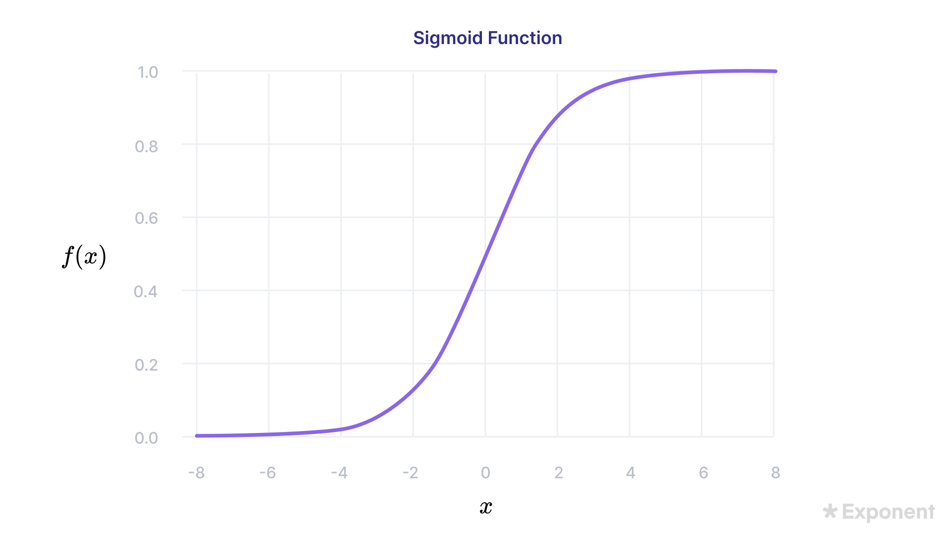
35. Explain Logistic Regression

Logistic regression is a classification algorithm that predicts binary outcomes (0 or 1).

It uses the same linear equation concept as linear regression, where the equation is:

Y=m1x1+m2x2+m3x3+...Y = m_1x_1 + m_2x_2 + m_3x_3 + ...Y=m1x1+m2x2+m3x3+...

In this equation, the model learns the coefficients (mmm) based on the features (xxx) to predict the target variable. Unlike linear regression, which fits a straight line across the data, logistic regression applies the logistic function (also called the sigmoid function) to map the linear output to a probability between 0 and 1.

This is more suitable for classification tasks, where the target variables consist of binary values (1 or 0).

If the predicted probability is greater than 0.5, the model classifies the output as 1; otherwise, it classifies it as 0. The threshold can be adjusted depending on the use case.

Learn more about the sigmoid function in logistic regression.

36. Explain Batch, Mini-Batch, and Stochastic Gradient Descent

Gradient Descent is an optimization technique that updates model parameters (weights) iteratively. The update process can be done in the following ways:

Batch Gradient Descent:
- The entire dataset calculates the gradient, and the weights are updated in a single step.
- Pros: Stable and points directly toward the global minimum.
- Cons: Slow, especially with large datasets, as the entire dataset is processed in each iteration.
Mini-Batch Gradient Descent:
- The dataset is divided into smaller batches, and the weights are updated after the gradient is calculated for each mini-batch.
- Pros: Faster and more efficient than batch gradient descent and reasonably stable.
- Cons: It may still not be as stable as batch gradient descent, but it is a good trade-off between speed and stability.
Stochastic Gradient Descent (SGD):
- Instead of processing the entire dataset or batches, weights are updated after computing the gradient for each training example.
- Pros: Extremely efficient for large datasets.
- Cons: Highly unstable, may lead to fluctuations, and might not converge to the global minimum.

37. Explain Classification and Regression

Classification:
- Classification algorithms predict discrete class labels. For example, the model predicts either 0 or 1 in binary classification, corresponding to two possible classes.
- Example: Predict whether an email is spam (1) or not (0).
Regression:
- Regression algorithms predict continuous values. The output is a real number, such as predicting the price of a house.
- Example: Predicting the selling price of a house based on features like size, location, and number of bedrooms.

38. Explain the Bias-Variance Tradeoff

Bias refers to the error introduced by simplifying the model's assumptions. A model with high bias tends to underfit the data, failing to capture the underlying patterns in training and test datasets.
Variance refers to the model's sensitivity to small fluctuations in the training data. A model with high variance tends to overfit the training data, performing well on the training set but poorly on the test set.

ℹ️

Practice answering this question. "Explain the bias-variance tradeoff."

The bias-variance tradeoff describes the challenge of balancing underfitting and overfitting.

A well-tuned model minimizes both bias and variance to achieve good performance on both the training and test datasets.

39. Explain Overfitting. How do you diagnose it?

Overfitting occurs when a model learns the noise and details of the training data so well that it negatively affects its performance on new data. An overfitted model performs well on the training set but poorly on test data or unseen examples.

How to diagnose overfitting:

The model shows excellent performance on the training set but poor performance on the test set.

How to prevent overfitting:

Simplify the model: Reduce the complexity of the model by reducing the number of layers or parameters in neural networks.
Feature reduction: Limit the number of features used in training to avoid irrelevant or noisy data.
Regularization: Apply techniques like L1 or L2 regularization to penalize complex models.
Cross-validation: Use cross-validation to evaluate the model on multiple subsets of the data.

40. How is AUC calculated? What are good values for AUC?

The Area Under the Curve (AUC) is a metric derived from the Receiver Operating Characteristic (ROC) curve. The ROC curve plots the True Positive Rate (Recall) against the False Positive Rate at various classification thresholds. The AUC measures the entire two-dimensional area under the ROC curve.

AUC values range from 0 to 1:
- An AUC of 0.5 means the model is no better than random guessing.
- AUC values between 0.7 and 0.9 are considered good, as they indicate the model can effectively distinguish between positive and negative classes.
- AUC values above 0.9 may suggest overfitting, where the model performs too well on the training data but might not generalize to unseen data.

In general, AUC helps evaluate how well the model ranks positive instances over negative instances across different threshold levels.

Interview Tips

It is impossible to cover all the possible questions since data science is a broad and varied interview type!

Explore our data science interview course's dozens of mock interviews and practice lessons.
Schedule a free mock interview session to practice answering questions with peers.
Get interviewing coaching from scientists at top companies.

Good luck with your upcoming DS interview!

Top Data Science Interview Questions and Answers (2026 Guide)

Statistics and Experimentation

What to expect

1. What are the measures of central tendency? Explain the significance of each.

2. In a positively skewed distribution, which measure of central tendency would likely be larger: the mean or the median? Why?

3. Explain the concept of correlation between two variables. How would you interpret a correlation value of +0.8?

4. How would you detect outliers in your data?

5. Design a hypothesis test.

6. Can you explain a p-value?

7. What's the difference between a Type I and a Type II error?

8. What's the central limit theorem, and how does it relate to hypothesis testing?

9. What does the confidence level mean when building a confidence interval?

Data Communication and Case Studies

10. Walk us through one of your most exciting data science projects.

11. How would you investigate a sudden viewer drop at Meta?

12. How would you use data to help Snap Engineering measure, evaluate, and improve phone camera speed?

Python

13. Given the DataFrame below, write a solution to fetch the three lowest-earning employees, including their IDs, names, and salaries.

14. Given a set of related DataFrames (described in the diagram below), write a solution to fetch the total transaction revenue per user city, ordered by descending revenue (in USD).

users

transactions

products

product_lines

exchange_rate

16. Given the DataFrame format below, write a function to identify the user who liked a post the quickest after logging in.

17. You have a user behavior log, but some records are duplicated, and some timestamps are missing. Since the logs are recorded chronologically, remove duplicates and fill in missing timestamps by interpolating the data.

SQL

18. How do you use a GROUP BY clause in SQL? What are some common aggregate functions used with GROUP BY?

19. What is a JOIN statement in SQL? Explain the different types of JOINS.

20. Write SQL code to show the total number of successful posts per user type in the current month (assumed to be November 2023).

22. What are window functions in SQL? Explain their syntax and usage.

23. Order departments by revenue over the last 12 months, showing department_name and total_revenue.

24. Write an SQL query to calculate the total transaction value in USD for the product line "Telephones" and return it as total_amount_in_dollars. You will need to convert non-USD amounts using the exchange rate and ensure proper scaling of the values.

25. Given the orders table, write an SQL query that returns the order_id, status, start_date, and end_date for each status period of an order. If a status is the first for that order, end_date should be NULL.

ML Coding

26. Write a function to simulate flipping a biased coin 20 times in each of 1,000 simulations, where each flip has a 20% chance of landing heads. Then, create a histogram showing the distribution of the number of heads observed in these 1,000 simulations.

27. Implement the KMeans clustering algorithm from scratch in Python.

28. Implement a 2D convolutional filter in Python.

29. How do you split up a machine learning dataset for training, evaluation, and testing?

ML Concepts

30. What are some common transformations for categorical data?

31. What is an imbalanced dataset? How can you address it?

32. How do splits occur in a decision tree?

33. When is accuracy a good or bad metric for evaluating a model?

34. How is MSE calculated, and when is it not a good metric?

35. Explain Logistic Regression

36. Explain Batch, Mini-Batch, and Stochastic Gradient Descent

37. Explain Classification and Regression

38. Explain the Bias-Variance Tradeoff

39. Explain Overfitting. How do you diagnose it?

40. How is AUC calculated? What are good values for AUC?

Interview Tips

Browse data scientist interview questions

Book time with a Data Scientist coach

Learn everything you need to ace your data science interviews.

Related Courses

Data Science Interview Prep

SQL Interviews

Related Blog Posts

15 Teleconferencing Tips for a Successful Remote Interview

Data Scientist vs. Data Analyst: Key Differences and Career Insights

The 5 Best Data Science Bootcamps

Transitioning From Data Analyst to Data Scientist

23. Order departments by revenue over the last 12 months, showing `department_name` and `total_revenue`.

24. Write an SQL query to calculate the total transaction value in USD for the product line "Telephones" and return it as `total_amount_in_dollars`. You will need to convert non-USD amounts using the exchange rate and ensure proper scaling of the values.

25. Given the `orders` table, write an SQL query that returns the `order_id`, `status`, `start_date`, and `end_date` for each status period of an order. If a status is the first for that order, `end_date` should be `NULL`.